When investigating a given system's trajectories and dynamics it
is often not intuitive how the system generally behaves. Even after
solving the state space and finding the eigenvalues and eigenvectors that
give information about the stability, it is still hard to visualize what
is occurring for a given set of trajectories.
In the special case of second-order systems, a phase portrait is particularly
useful. It plots the system trajectories as contours over a timespan along the X and Y axes
which respectively represent the first and second order of the state space. In the
case of nonlinear systems, phase portraits are particularly useful
because they do no require any linearization or elimination of nonlinear terms.
The phase portraits is able to perfectly capture all of the nonlinear trajectories
and display them in a way that would be otherwise difficult.
The simple pendulum is a great example of a second-order nonlinear system that can
be easily visualized by the phase portrait. The simple pendulum is often linearized using
the small-angle approximation and converted into a linear form of zdot = A*z where
A is a matrix of scalars. Instead, the phase portrait method
leaves the simple pendulum state space in its nonlinear form as sin(θ).
It is worth noting that the inherent limitation of phase portraits is that they only
applicable in second-order or lower systems. However, it cannot be asserted
enough how effective phase portraits are at giving quick analysis for even
highly-nonlinear systems.
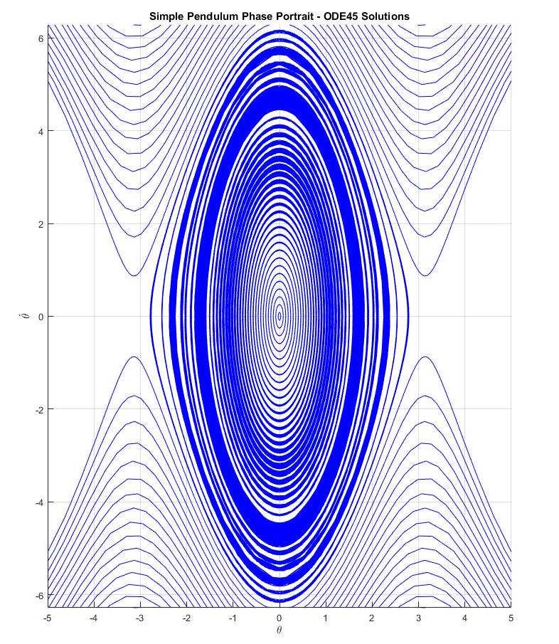
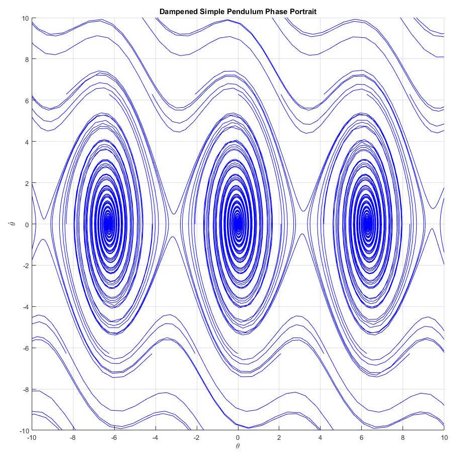
The code below provide phase portraits for various dampened and undampened
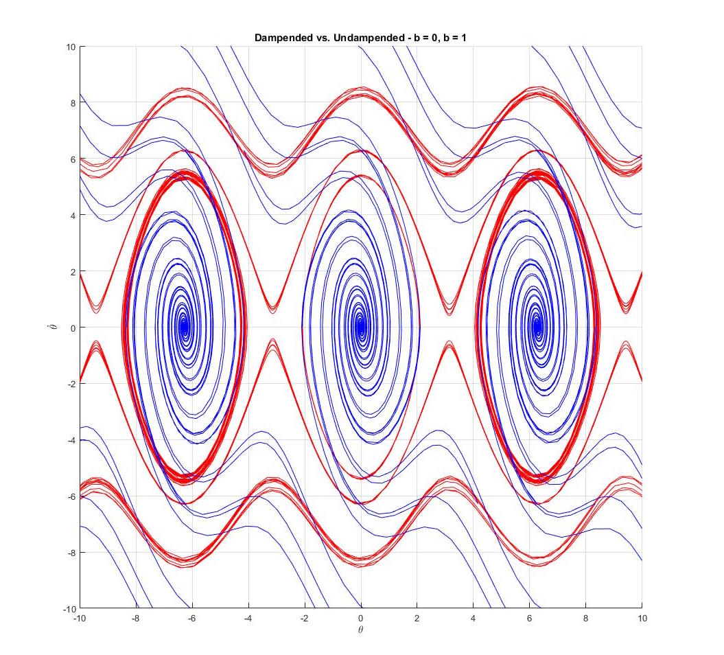
simple pendulum scenarios. Notice how the dampened trajectories converge
to a point while the undampened ones form concentric contours, formally known as
limit cycles.
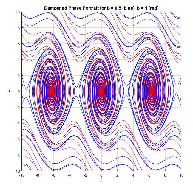
Also, notice how for the larger dampening coefficient, the trajectories converge to a point
much quicker, with fewer rotations around. This reflects our intution that a
pendulum with more friction (a larger dampening coefficient) will come to rest faster.
Similarly, the limit cylces formed
in the undampened figures show that without any friction, the pendulum will continue
to swing around the equilibrium point forever. It is clear why phase portraits
are a powerful tool for analyzing nonlinear systems, read more about
them here.
            % Script for Plotting the Phase Portrait of a Nonlinear Pendulum

            % init system and states
            g = 9.81;
            L = 1;
            ss = @(t,THETA) [THETA(2); -g./L*sin(THETA(1))];
            THETA1 = linspace(-2*pi,2*pi,50);
            THETA2 = linspace(-2*pi,2*pi,25);

            % Generate Meshgrid for numerically solving
            [x,y] = meshgrid(THETA1,THETA2);
            size(x)
            size(y)

            % Establish U and V vectors
            u = zeros(size(x));
            v = zeros(size(y));

            % Init Loop over Vector field to compute Derivatives
            t = 0;
            for i = 1:numel(x)
                Theta_d = ss(t,[x(i); y(i)]);
                u(i) = Theta_d(1);
                v(i) = Theta_d(2);
                Mag = sqrt(u(i)^2+v(i)^2);
                %u(i) = u(i)/Mag;
                %v(i) = v(i)/Mag;
            end

            %Plot our vector field
            quiver(x,y,u,v,'r'); figure(gcf)
            xlabel('${\theta}$','interpreter','latex')
            ylabel('$\dot{\theta}$','interpreter','latex')
            axis tight equal;

            hold on

            % Plotting Solutions for Comparison
            for THETA_sol = linspace(-4*pi,4*pi,150)
                [ts,ys] = ode45(ss,[0,50],[0;THETA_sol]);
                plot(ys(:,1),ys(:,2),'b')
                plot(-ys(:,1),ys(:,2),'b')
                %plot(ys(1,1),ys(1,2),'bo') %start of contour
                %plot(ys(end,1),ys(end,2),'ks') %end of contour
            end

            axis([-5 5 -2*pi 2*pi])
            grid on


            hold off
            % Script for Plotting the Phase Portrait of a Dampened Nonlinear Pendulum
            % Change the state space to include "b" dampening coefficient

            % init system and states
            g = 9.81;
            L = 1;
            b = 1;
            ss = @(t,THETA) [THETA(2); -b.*THETA(2)-g./L*sin(THETA(1))];
            THETA1 = linspace(-2*pi,2*pi,50);
            THETA2 = linspace(-2*pi,2*pi,25);